Interpolation#
강좌: 수치해석
개요#
Interpolation (보간): 데이터들 사이에 있는 중간값을 산출
Extrapolation (외삽): 데이터들을 바탕으로 그 밖에 있는 값을 추정

Fig. 13 Interpolation (from Wikipedia)#
Regression (회귀): 데이터들에 적합한 함수 산출
%matplotlib inline
from matplotlib import pyplot as plt

import numpy as np

plt.style.use('ggplot')
plt.rcParams['figure.dpi'] = 150
Newton의 제차분 보간 다항식 (divided-difference interpolating polynomial)#
Linear Interoplation#
\(x=x_0, x_1\) 두 지점에서 함수 값 \(f(x_0), f(x_1)\)을 알고 있을 때
선형 보간 함수 \(f_1(x)\)
정리하면
예제#
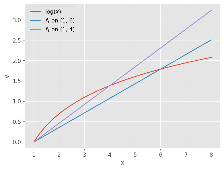
아래 테이블을 이용하여 \(\log(2)\) 값 보간
\(x\) |
1 |
4 |
6 |
|---|---|---|---|
\(\log(x)\) |
0.0 |
1.386294 |
1.781759 |
\(x_0=1\), \(x_1=6\) 일 때
def fi1(x0, x1, f0, f1):
    fi = lambda x : f0 + (f1 - f0) / (x1 - x0)*(x-x0)

    return fi
x0, x1 = 1, 6
f0, f1 = np.log([x0, x1])

f16 = fi1(x0, x1, f0, f1)
f16(2)
0.358351893845611
\(x_0=1\), \(x_1=4\) 일 때
x0, x1 = 1, 4
f0, f1 = np.log([x0, x1])

f14 = fi1(x0, x1, f0, f1)
f14(2)
0.46209812037329684
x = np.linspace(1, 8, 81)
plt.plot(x, np.log(x))
plt.plot(x, f16(x))
plt.plot(x, f14(x))

plt.xlabel('x')
plt.ylabel('y')
plt.legend(["$\log(x)$", "$f_1$ on (1, 6)", "$f_1$ on (1, 4)"])
<matplotlib.legend.Legend at 0x7fa4e2927610>
# Relative Error
fexact = np.log(2)
print("True relative error of f16: {:.4f}%".format(abs((f16(2) - fexact)/fexact)*100))
print("True relative error of f14: {:.4f}%".format(abs((f14(2) - fexact)/fexact)*100))
True relative error of f16: 48.3007%
True relative error of f14: 33.3333%
Quadratic Interoplation#
\(x=x_0, x_1, x_2\) 세 지점에서 함수 값 \(f(x_0), f(x_1), f(x_2)\)을 알고 있을 때
앞선 선형 보간 함수 형태로 부터
2차 다항식 \(f_2(x)\)
함수 값을 적용하면
\(f_2(x_0) = f(x_0)\)
\[ f_2(x_0) = b_0 = f(x_0) \]\(f_2(x_1) = f(x_1)\)
\[ f_2(x_1) = b_0 + b_1 (x_1 - x_0) = f(x_1) \]이전 결과 대입
\[ b_1 = \frac{f(x_1) - f(x_0)}{x_1 - x_0}. \]
\(f_2(x_2) = f(x_2)\)
\[ f_2(x_2) = b_0 + b_1 (x_2 - x_0) + b_2 (x_2 - x_0) (x_2 - x_1) = f(x_2) \]이전 결과 대입
\[ b_2 = \frac{\frac{f(x_2) - f(x_1)}{x_2 - x_1} - \frac{f(x_1) - f(x_0)}{x_1 - x_0}}{x_2 - x_0} \]
이전 예제#
def fi2(x0, x1, x2, f0, f1, f2):
    b0 = f0
    b1 = (f1 - f0) / (x1 - x0)
    b2 = ((f2 - f1) / (x2 - x1) - b1) / (x2 - x0)

    fi = lambda x : b0 + b1*(x-x0) + b2*(x-x0)*(x-x1)

    return fi
x0, x1, x2 = 1, 4, 6
f0, f1, f2 = np.log([x0, x1, x2])

f146 = fi2(x0, x1, x2, f0, f1, f2)
f146(2)
0.5658443469009827
x = np.linspace(1, 8, 81)
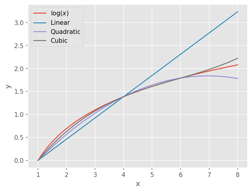
plt.plot(x, np.log(x))
plt.plot(x, f14(x))
plt.plot(x, f146(x))
plt.xlabel('x')
plt.ylabel('y')
plt.legend(["$\log(x)$", "Linear", "Quadratic"])
<matplotlib.legend.Legend at 0x7fa4e256d550>

# Relative Error
fexact = np.log(2)
print("True relative error of f16: {:.4f}%".format(abs((f146(2) - fexact)/fexact)*100))
True relative error of f16: 18.3659%
General form#
\((n+1)\) 개의 데이터로 \(n\) 차 보간 다항식
\[ f_n (x) = b_0 + b_1 (x - x_0) + ... + b_n(x - x_0)(x - x_1)...(x - x_{n-1}) \]계수
\[\begin{split} \begin{align} b_0 & = f(x_0) \\ b_1 & = f[x_1, x_0] \\ b_2 & = f[x_2, x_1, x_0] \\ ... \\ b_n & = f[x_n, x_{n-1}, ..., x_0] \end{align} \end{split}\]유한 제차분
\[\begin{split} \begin{align} f[x_i, x_j] &= \frac{f(x_i) - f(x_j)}{x_i - x_j} \\ f[x_i, x_j, x_k] &= \frac{f[x_i, x_j] - f[x_j, x_k]}{x_i - x_k} \\ ... \\ f[x_n, x_{n-1},...,x_1, x_0] &= \frac{f[x_n, x_{n-1},...,x_1] - f[x_{n-1}, x_{n-2},...,x_0]}{x_n - x_0} \end{align} \end{split}\]
이전 예제#
\(x_3 = 5\) 인 점을 추가해서 3차 보간식 구성하시오.
x0, x1, x2, x3 = 1,4,5,6
f0, f1, f2, f3 = np.log([x0, x1, x2, x3])
def difference(xi, xj, fi ,fj):
    # 1차 유한 차분
    return (fi - fj) / (xi - xj)

# 반복적으로 재차분
df1 = difference(x1, x0, f1, f0)
df2 = difference(x2, x1, f2, f1)
df3 = difference(x3, x2, f3, f2)

ddf1 = difference(x2, x0, df2, df1)
ddf2 = difference(x3, x1, df3, df2)

dddf1 = difference(x3, x0, ddf2, ddf1)
fi = lambda x: f0 + df1*(x-x0) + ddf1*(x-x0)*(x-x1) + dddf1*(x-x0)*(x-x1)*(x-x2)
fi(2)
0.6287685789084135
x = np.linspace(1, 8, 81)
plt.plot(x, np.log(x))
plt.plot(x, f14(x))
plt.plot(x, f146(x))
plt.plot(x, fi(x))

plt.xlabel('x')
plt.ylabel('y')
plt.legend(["$\log(x)$", "Linear", "Quadratic", "Cubic"])
<matplotlib.legend.Legend at 0x7fa4e0ade110>
# Relative Error
fexact = np.log(2)
print("True relative error of cubic interpolation: {:.4f}%".format(abs((fi(2) - fexact)/fexact)*100))
True relative error of cubic interpolation: 9.2879%
DIY#
n차 Newton 제차분 보간 다항식을 구하는 함수를 구성하시오.
미리 필요한 제차분을 구해서 저장하여 보간함수를 구성하시오.
제차분을 구하는 Recursive 함수를 구성하여 보간함수를 구성하시오.
Lagrange Interpolating Polynomial#
제차분을 사용하지 않도록 Newton 다항식을 재구성한 식
\[ f_n(x) = \sum_{i=0}^n L_i(x) f(x_i). \]\(L_i(x)\)
\[ L_i(x) = \Pi_{j \neq i}^n \frac{x-x_j}{x_i - x_j} \]\(L_i(x_j) = \delta_{ij}\).
선형 보간 다항식 예제
\[ f_1 (x) = \frac{x - x_1}{x_0 - x_1} f(x_0) + \frac{x - x_0}{x_1 - x_0} f(x_1) \]
위 예제를 1, 2차 다항식 구성#
# Linear
x = 2
xdata = [1, 4]
fdata = np.log(xdata)

f = 0
for xi, fi in zip(xdata, fdata):
    # Compute Li
    Li = 1
    for xj in xdata:
        if xi != xj:
            Li *= (x- xj)/(xi - xj)

    f += Li*fi

print(f)
0.46209812037329684
# Cubic
x = 2
xdata = [1, 4, 6]
fdata = np.log(xdata)

f = 0
for xi, fi in zip(xdata, fdata):
    # Compute Li
    Li = 1
    for xj in xdata:
        if xi != xj:
            Li *= (x- xj)/(xi - xj)

    f += Li*fi

print(f)
0.5658443469009826
DIY#
n차 Lagrange보간 다항식을 구하는 함수를 구성하시오.
For loop를 List Comprehesion 으로 구성해보시오.
Spline 보간법 (Interpolation)#
개요#
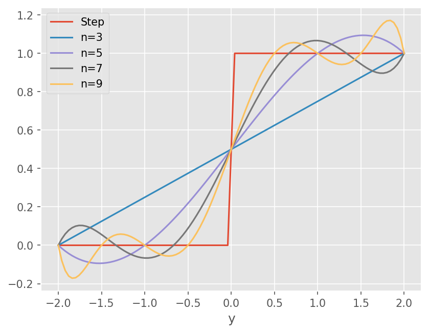
Gibbs phenomena
고차 내삽은 항상 정확한가?
Step function
x = np.linspace(-2, 2, 101)
stepf = lambda x: (1+np.tanh(1e8*x))/2
fs = []
for n in [3, 5, 7, 9]:
    xdata = np.linspace(-2, 2, n)
    fdata = stepf(xdata)

    f = 0
    for xi, fi in zip(xdata, fdata):
        # Compute Li
        Li = 1
        for xj in xdata:
            if xi != xj:
                Li *= (x- xj)/(xi - xj)

        f += Li*fi

    fs.append(f)
plt.plot(x, stepf(x))

for fi in fs:
    plt.plot(x, fi)

plt.xlabel('x')
plt.xlabel('y')
plt.legend([
    'Step', 'n=3', 'n=5', 'n=7', 'n=9'
])
<matplotlib.legend.Legend at 0x7fa4e043d710>
Piecewise interpolation, smooth
Linear spline#
구간 내에서 선형 보간
Continuity

Fig. 14 Linear Spline (from Wikipedia)#
각 구간은 선형 분포
\[ s_i(x) = a_i + b_i(x-x_i) \]연속분포 만족
\[\begin{split} \begin{align} a_i &= f_i \\ b_i & = \frac{f_{i+1} - f_i}{x_{i+1} - x_i} \end{align} \end{split}\]Linear Newton or Lagrange interpolation
knots: 두 스플라인이 만나는 점
기울기가 급격히 변함
예제#
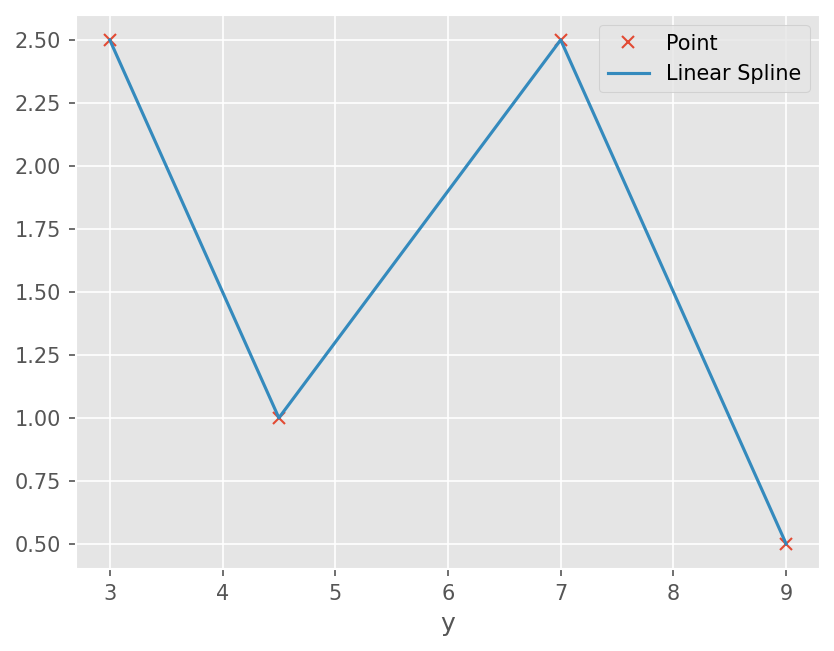
다음 분포에 대한 선형 Spline 을 구하시오
i |
\(x_i\) |
\(f_i\) |
|---|---|---|
1 |
3.0 |
2.5 |
2 |
4.5 |
1.0 |
3 |
7.0 |
2.5 |
4 |
9.0 |
0.5 |
xdata = np.array([3, 4.5, 7.0, 9.0])
fdata = np.array([2.5, 1.0, 2.5, 0.5])
xs = np.linspace(3, 9, 61)

s = []
for x in xs:
    for xf, xb, ff, fb in zip(xdata[:-1], xdata[1:], fdata[:-1], fdata[1:]):
        # Left
        if abs(x - xf) < 1e-12:
            si = ff
            s.append(si)
            break
        # Right
        elif abs(x - xb) < 1e-12:
            si = fb
            s.append(si)
            break
        # Between
        elif (x - xf)*(x - xb) < 0:
            si = ff + (fb - ff)/(xb - xf)*(x - xf)
            s.append(si)
            break
plt.plot(xdata, fdata, linestyle='', marker='x')
plt.plot(xs, s)

plt.xlabel('x')
plt.xlabel('y')
plt.legend(['Point', 'Linear Spline'])
<matplotlib.legend.Legend at 0x7fa4e04876d0>
2차 스플라인#
구간 내 2차함수
내부 절점에서 1차 도함수가 연속

Fig. 15 Quadtratic Spline (from Wikipedia)#
각 구간은 2차 함수
\[\begin{split}\begin{align} s_i(x) &= a_i + b_i(x-x_i) + c_i (x - x_i)^2 \\ s'_i(x) &= b_i + 2c_i (x - x_i) \end{align} \end{split}\]연속조건 \(s_i(x_i) = f_i\)
\[ a_i = f_i \]절점에서 값이 같아야 함 \(s_i(x_{i+1}) = s_{i+1}(x_{i+1}) = f_{i+1}\)
\[ f_i + b_i h_i + c_i h_i^2 = f_{i+1}, h_i = x_{i+1} - x_i \]절점에서 1차 도함수 같음 \(s'_i(x_{i+1}) = s'_{i+1}(x_{i+1})\)
\[ b_i + 2c_i h_i= b_{i+1} \]첫점째 점에서 2차 도함수 0
\[ c_0 = 0 \]
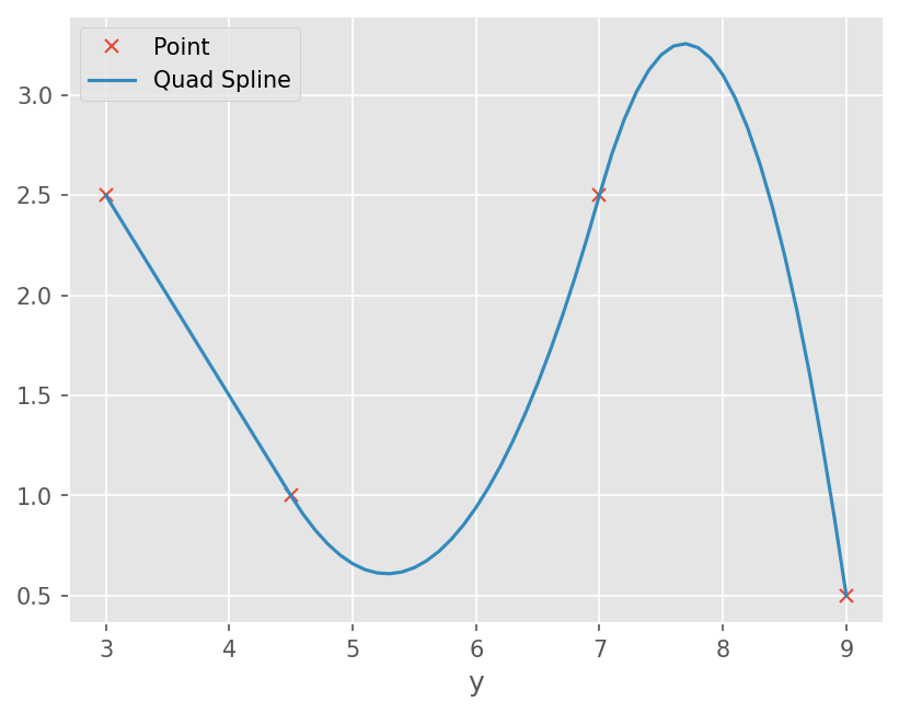
예제#
앞선 분포에 대한 Quadratic Spline 을 구하시오.
4개의 데이터와 3개의 구간
미지수 \(b_0, b_1, c_1, b_2, c_2\)
선형 방정식 구현
\[\begin{split} \begin{bmatrix} h_0& 0 & 0 & 0 & 0 \\ 0 & h_1 & h_1^2 & 0 & 0 \\ 0 & 0 & 0 & h_2 & h_2^2 \\ 1 & -1 & 0 & 0 & 0 \\ 0 & 1 & 2h_1 & -1 & 0 \end{bmatrix} \begin{bmatrix} b_0 \\ b_1 \\ c_1 \\ b_2 \\ c_2 \end{bmatrix} = \begin{bmatrix} \Delta f_1 \\ \Delta f_2 \\ \Delta f_3 \\ 0 \\ 0 \end{bmatrix} \end{split}\]
xdata = np.array([3, 4.5, 7.0, 9.0])
fdata = np.array([2.5, 1.0, 2.5, 0.5])

h = np.diff(xdata)
df = np.diff(fdata)

A = np.array([
    [h[0], 0, 0, 0, 0],
    [0, h[1], h[1]**2, 0 ,0],
    [0, 0, 0, h[2], h[2]**2],
    [1, -1, 0, 0, 0],
    [0, 1, 2*h[1], -1, 0]
])

ff = np.array([df[0], df[1], df[2], 0, 0])

# Solve equations
x = np.linalg.solve(A, ff)

b= np.array([x[0], *x[1::2]])
c = np.array([0, *x[2::2]])
xs = np.linspace(3, 9, 61)

s = []
for x in xs:
    for i, (xf, xb) in enumerate(zip(xdata[:-1], xdata[1:])):
        # Left
        if abs(x - xf) < 1e-12:
            si = fdata[i]
            s.append(si)
            break
        # Right
        elif abs(x - xb) < 1e-12:
            si = fdata[i+1]
            s.append(si)
            break
        elif (x - xf)*(x- xb) < 0:
            bi, ci = b[i], c[i]
            si = fdata[i] + bi*(x- xf) + ci*(x - xf)**2
            s.append(si)
            break
plt.plot(xdata, fdata, linestyle='', marker='x')
plt.plot(xs, s)

plt.xlabel('x')
plt.xlabel('y')
plt.legend(['Point', 'Quad Spline'])
<matplotlib.legend.Legend at 0x7fa4e040f6d0>
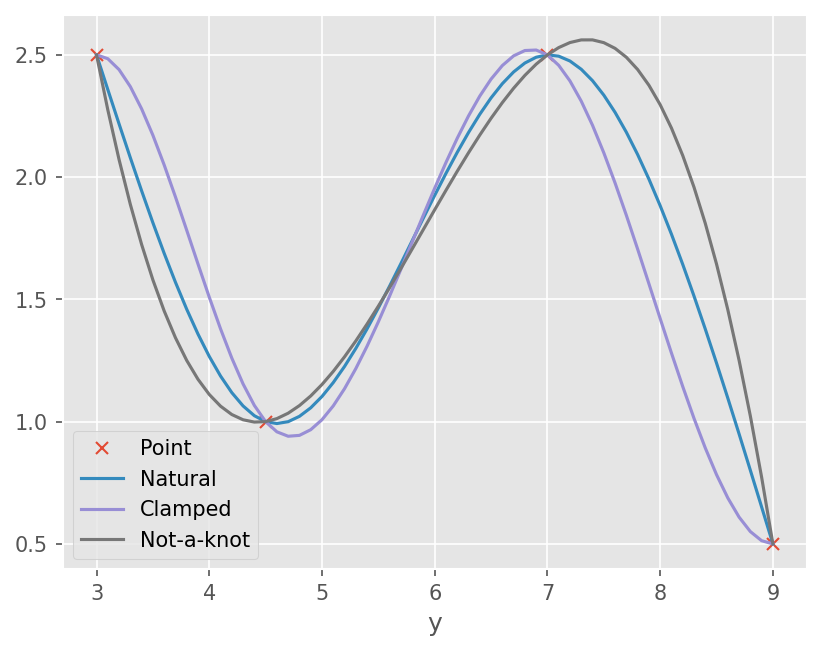
3차 스플라인#
가장 널리 사용됨
구간 내 3차함수
내부 절점에서 1차 도함수가 연속
내부 절점에서 2차 도함수가 연속
양 끝 구간
Natural spline 처음, 마지막 절점: 2차 도함수를 0
Clamped: 양 끝단 고정 (1차 도함수 0)
Not-a-knot: 처음 두 구간과 마지막 두구간에 하나의 3차 다항식 (3차 도함수 연속)

Fig. 16 Cubic Spline (from Wikipedia)#
from scipy.interpolate import CubicSpline

fnatural = CubicSpline(xdata, fdata, bc_type='natural')
fclamped = CubicSpline(xdata, fdata, bc_type='clamped')
fnotaknot = CubicSpline(xdata, fdata, bc_type='not-a-knot')
xs = np.linspace(3, 9, 61)

plt.plot(xdata, fdata, linestyle='', marker='x')
plt.plot(xs, fnatural(xs))
plt.plot(xs, fclamped(xs))
plt.plot(xs, fnotaknot(xs))

plt.xlabel('x')
plt.xlabel('y')
plt.legend(['Point', 'Natural', 'Clamped', 'Not-a-knot'])
<matplotlib.legend.Legend at 0x7fa4daf2e110>
Scipy 활용#
Scipy 에는 다양한 내삽 함수를 제공한다.
scipy.interpolate모듈